Abstract

The paper presents the comprehensive assessment of the resolution capacity of MRL5 radar ornithological station developed in Israel. Theoretical calculations, as well as experimental testing and field experience enable the authors to evaluate the station’s performance and to suggest new directions of its potential development.

Key words: Bird migration, birds, radar ornithology, radars.

1. Introduction.

MRL5(Is) is a radar ornithological station developed in Israel on the basis of МRL-5 meteorological radar. The system performs computer-controlled bird monitoring 24 x 7 and enables to obtain, at the interval of 15- 20 minutes, updated information on bird flights over large areas within the hemispherical coverage regardless of weather conditions. MRL-5 is able to reliably detect echoes of birds as big as storks at the distance of 90 km. км. The computer-controlled system is able to select bird echoes and plot ornithological charts for distances up to 60 km. This restriction in distance is accounted for by several reasons, namely, a) computation rates; b) large corpora of data to undergo sophisticated and complicated analysis and c) restricted time intervals set by aviation services for the ornithological charts to be regularly updated.

The technical parameters of the station, its problem-solving algorithms and results obtained in years-long experience in bird monitoring over Central Israel are presented in a number of studies (Dinevich, 2009; Dinevich et al., 2000; Dinevich et al., 2001; Leshem et al., 2003; Dinevich et al., 2003; Dinevich et al., 2004; Dinevich et al., 2005; Dinevich and Leshem, 2007; Dinevich and Leshem, 2008).

The purpose of the present paper is to assess the accuracy of results obtained with MRL5(Is) and to suggest potential directions of the further development of the station. The data to be assessed were obtained, according to our Customer’s request, in order to provide information on bird migration that is of significant importance for ornithologists and ecologists, as well as for various aviation services. The observations were performed in autumn and in spring, in daylight (from 08.00 a.m. to 17.00 p.m.) over the year of 2009 and at nighttime (from 18.00 p.m. to 0.6.00 a.m.) over the year of 2010. Below, the analysis of the these observations is presented alongside with the assessment of the MRL5(Is) station accuracy.

2. Radar Equation for a bird flock

A big bird flock is a dispersed multiple radar target whose characteristics mostly resemble those of clouds and precipitation. MRL-5 has a narrow pencil-like beam and is capable of detecting at high accuracy both the location and the flight speed of a multiple (dispersed) radar target or a single target (Abshayev et al. ,1980), including birds (Dinevich and Leshem, 2008).

While deriving Radar Equation, we assume that the antenna beam is of symmetrical cone-like shape.

The beam width for an antenna is determined by the angular width of the cone at the level of half-power of the probing signal. For a single bird or a small bird flock totally radar-covered within the scanning reflecting zone (see below) the well-known radar equation is valid

,  (1 )

where is the power at the receiver entry, is the transmitter power, is the antenna power gain, is the wavelength, is the scattering cross section (SCS) of the target and is the total attenuation of the waveguide transmission line.

The attenuation within clouds and precipitation is not taken into account since birds are unlikely to fly under conditions of heavy rain or clouds.

Substituting the known values for dependencies of the antenna power gain on its aperture (the actually used antenna square) and the dependencies of the antenna power gain of its beamwidth , we can write several equivalent expressions for the radar equation.

SCS of a single bird of dimensions big enough to be comparable with the wavelength is approximately equal to its cross section area as seen at the point of the radar (plumage not taken into account). A bird’s SCS depends on the flight stage and the flight course relative respect to the radar (Ganja et al., 1991; Chernikov, 1979). These dependencies can be utilized for the purposes of bird species determination. Fig. 1 (a, b) present bird SCSs measured by different authors at various wavelengths (3.2 cm, 5.0 cm, 10.0 cm and 71,5 cm). For the sake of comparison, the figure also shows SCS values obtained by other authors by means of radars of other types (Chernikov, 1979). To calculate s, we used the formulas suggested by Stepanenko (1973):

for λ=3,2 cm, s cm2 = 0,6·10^-24 10 ^0,1n R⁴,

for λ=10 cm sсm2 = 0,28·10^-25 10 ^0,1n R⁴

where n is the radar reflectivity of the experimental target measured in dB and R is the distance to the target (in meters). The coefficients in the formulas are calculated based on the constant parameters of the antenna, the receivers and the transmitters. The principle for bird echo isolation utilized in this study is described in (Dinevich et al, 2001). Fig. 1(a) shows that the SCS values on the second channel are higher than those on the first channel, thus meaning that our findings are close to the results obtained by other authors (Chernikov 1979).

In some cases the authors classified the echoes with the corresponding values to insect echoes (Fig. 1(b)). Their SCSc values at 3 cm wavelength are higher that those at the 10 cm wavelength. In these cases visual observations showed large presence of insects near the ground (midges, moths, mosquitoes etc) well seen in the light of street lamps, car headlights and even in darkness at short distances). According to radiosonde data, the ground air in these cases was characterized by higher humidity, with a weak wind directed to west-northwest.

For example, in case study on October 25 at 21.30 (fig. 1b - (marked with *) the first inversion level was determined at the height of 800-1200m. The moon was seen through sparse light. At those heights, at both MRL-5 channels one could see a weak but vast echo from an invisible atmospheric inhomogeneity about 500 m thick. This may suggest a possible presence of vertical air flows in the subinversion air level, that triggered accumulation of various admixtures including insects. A specific feature of this echo was the difference in its differential reflectivity values measured at its upper level vs. its bottom level.

The differential reflectivity was calculated with the help of the expression dP=P_II/P⊥, where dP (the differential reflectivity) is a nondimensional quantity, P_II is the power of the reflected signal measured in megawatt (a horizontal polarization wave was both received and radiated) and P⊥ is the power of the reflected signal measured in megawatt (a vertical polarization wave was both received and radiated). The polarization is altered pulse by pulse. At the repetition rate of 500 pulses per second the frequency of polarization alteration is 1/500 sec. We assume that during such a short period of time the targets we study (clouds, atmospheric inhomogeneities and birds) cannot change their status.

The signal was averaged over approximately 250 pulses. The values of the differential reflectivity at the upper part of the echoes was close to unity (or 0 dB) which is typical of the reflection from cloud particles or of boundaries of atmospheric layers with high temperature-humidity gradient (Shupijatcky,1959, Chernikov and Shupiatsky,1967, Zrnic and Ryzhkov,1998). This can be accounted for by the isotropic reflectivity properties of atmospheric inhomogeneities (visually unobservable thermics or mesofronts), small-size spherical cloud drops that are chaotically oriented in the medium of small crystals (in our case, there can be no such crystals).

The differential reflectivity from the bottom part of the echo was >1 which is typical of non-spherical reflectors horizontally oriented in the space (Dinevich et al., 1994).

Thus suggests that the bottom part of the echo was formed not only due to the temperature-humidity gradient, but also due to the presence of horizontally oriented dipoles present within the subinversion layer; these dipoles can be only insects or oblong plant seeds. In addition, it should be emphasized that the echoes in all the cases shifted in the direction and at the speed of the wind at this level (according to the reading of the radio-probing closest in time). It allows us to conclude that that the echoes we observed on both channels in these observations were insect echoes. The SCS radar was always higher at the 3 cm wavelength that on the 10cm wavelength, which is in accordance with conclusions made by other researchers (Glover and Hardy, 1966; Chernikov, 1979).

Our observation results show that the 10cm channel is more efficient in detecting birds, yielding better results in both the number of detected birds and the detection distance in the same situation. Thus can be accounted for by the fact that the 10cm channel has a higher potential and a wider beam “catching" birds over a larger area. For this reason, we selected the second channel (λ=10 cm) for performing our bird monitoring.

Fig. 1(a,b) below demonstrates that the measured values of SCS match the data obtained by different authors, as cited by A. A. Chernikov (1979).

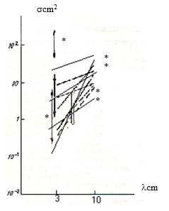
Fig. 1(a). The scattering cross-section of  birds on the 3 cm and 10 cm wavelengths.

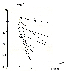
Fig 1(b). The scattering cross-section of insects on the 3 cm, 10 cm and 71.5 cm wavelengths.

Fig. 1 (a,b) shows SCSs for various bird and insect species measures at various wavelengths (3.2 cm, 5.0 cm, 10.0 cm and 71,5 cm) by different authors (Richardson and West, 2005; Houghton, 1964; Konrad, Hicks, 1966; Rinehart, 1966; Glover and Hardy, 1966; Hajovsky et al., 1966; Chernikov 1979) as well as by the authors of this paper (marked with *). The figure shows quite good agreement between the data. At wavelengths of 3 cm and 10 cm bird SCSs increase depending on the species dimensions. For insects (Fig.1 b) we see the reverse dependence on the wavelength.

For the purposes of this paper, its is enough to use the averaged data. Table 1 below presents the mean SCS for various bird species at the radar wavelength cm.

Table 1. Scattering cross-section (SCS) for various bird species according to calculations.

While deriving the Radar Equation for a big bird flock we based on the approach traditionally used for deriving the radar equation for a dispersed multiple target such as clouds and precipitation. This approach is related to the concept of reflecting area (Abshayev at al.,1984). With the reflecting signal being at a certain delay from the moment of probing, the delay being expressed as (where is the distance to the target and is the light speed), the volume of the reflectivity area is expressed as (where is the duration of the probing pulse). The radar beam being symmetrical, this volume has a cylinder-like shape having as its base a circle of radius and the height of . The axis of the cylinder is angled relative to the Earth surface, the angle being equal to the tilt angle of the antenna.

A typical structure of a cloud is significantly different from that of a bird flock. The typical thickness of a cloud is less than its horizontal dimension and is less than the diameter of the reflective area at smaller distances. Unlike clouds, birds usually fly in the daylight approximately at the same height, thus a bird flock forms a relatively thin horizontal layer. For this reason, the classic radar equation valid for clouds and precipitations (Abshayev, Kaplan and Kapitannikov, 1984) is not applicable for a big bird flock flying within a small height range.

The square of the area covered by a bird flock flying at the same height and getting entirely within the reflectivity area depends on the tilt angle. At small distances 

(2 )

while at large distances

  (2a )

The critical angle at which one should shift from (1) to (2) is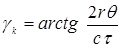. In case, formula (2) is valid, otherwise (2a) is to be applied.

As a rule, the tilt angle that allows to detect birds is less than the critical angle and close to zero angle, hence we can express the square of the layer as

  (3 )

Hereafter, we are going to use the expression (1) for the square of the layer.

In case a single bird is flying at the average distance from the next-flying birds and occupies the fraction of the square equal to, the number of birds simultaneously exposed to the radar radiation is . Using the obvious assumption that the signal from a bird flock is scattered incoherently, at the SCS value for a single bird as we obtain the SCS for the volume surrounding the bird as.

Substituting this value into formula (1) and using (3) for , we derive the radar equation for a bird flock flying at a large distance from the radar at the tilt angle close to zero

   (4 )

where the dependency is utilized in the right-hand equality.

For a bird flock seen at a significantly high tilt angle that is still less than the critical angle, the Radar Equation looks as

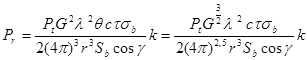            ( 4a )

Therefore, the power of the signal reflected from a bird flock is inversely proportional to the cube of the distance.

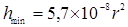
It should be noted that at night birds usually fly within a larger height range and at higher density within the radar scan. In this case the power of the signal reflected from a bird flock covering a certain volume is similar to the power of signal reflected from a cloud and thus is inversely proportional to r4.

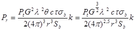
By way of example, we calculate here the power of signal received on the first MRL-5 channel, reflected from a flock of sparrows 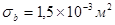flying at an average distance of 30 m from each other () at the height of 500 m and the distance from the radar of 30 km. The tilt angle at which the target is viewed is =2,90, and the critical angle is

= 310.

Therefore, one can apply the radar equation from (4).

Substituting the parameters of the MRL-5 first channel into (4), we obtain

= 3.2 cm, =0,5⁰=0,009,

, = 10^-6 microsec,

, and .

We obtain, which is a value by three orders of magnitude higher than which is the threshold sensitivity of the receiver . As can be seen from this example, the power of a received signal is not a factor restricting the distance of bird radar monitoring.

Using the Radar Equation for birds, we can, on the basis of a received signal, evaluate the complex parameter of specific SCS, i.e. SCS per a square unit of the bird-coved layer. If, in addition to the value, we have some data on the averaged distance between the next-flying birds, we can calculate the SCS for a single bird. And vice versa - if we have additional data on the SCS for a single bird, we can evaluate the distance between next-flying birds and thus evaluate the number of birds in the flock. The number of birds in a flock us an important parameter per se; SCS of a single bird enables to evaluate its size and thus determine its species with a certain probability. However, none of these parameters can be evaluated solely on the basis of the amplitude of a signal yielded by a single probing. By taking into account the specific geometric features characterizing flight patterns of various bird species (Shestakova, 1971), as well as various parameters of radar echo (fluctuation, polarization, two-wave mode, Doppler, spatial and temporal characteristics) we can evaluate several important ornithological parameters (Zavirucha et al., 1977; Dinevich et al., 1994; Ganja et al., 1991; Zrnic and Ryzhkov, 1998, Leshem et al., 2003). For example, it was shown (Dinevich et al. 2004) that analysis of fluctuation parameters of radar echo can enable isolating signals from single birds at high accuracy. Sound tracking of the fluctuations provides data on the changes in spatial orientation of the bird and the pattern of its wings flapping. On the basis of the Radar Equation formulated above, SCS of the bird can be measured , thus providing data on the bird’s size. These parameters alongside with the pattern of the bird’s movement in the space enable to determine its species (Shestakova, 1971; Dinevich and Leshem, 2007; Dinevich and Leshem, 2008; Doviak and Zrnic, 1984). By putting together the measurements of the radar reflectivity within each radar scan as well as the data on bird species and SCS, one can approximately assess the number of birds in a flock and their concentration within a certain space. However, a detailed analysis of this issue is beyond the scope of the paper.

3. Restrictions on the bird echo monitoring due to the curvature of the Earth

As was shown in the study (Abashev et al., 1984), the maximum range of vision (km) determined by the curvature of the Earth depends on the height of the radar location and the height of the target , thus

(5 )

In most cases, the height of the radar location is significantly lower than that of the target, thus making the first summand in (5) negligible:

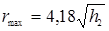(6 )

In the inverse formulation, this formula determines the maximum height (meters) at which a target is visible at a certain distance (kilometers)

(7 )

While determining the maximum range of vision on the basis of (5, 6, 7), the beam width is assumed to be small and it is supposed that the radar beam can be at zero angle relative to the Earth surface. However, at extremely small tilt angles the beam “gears” the Earth surface. This leads to a change in the amplitude of the received signal, and what is more significant, to emergence of ground clutter reflections (those from hills, woods, buildings and other installations). The bird signal being relatively weak, those ground clutter reflections disguise it making it indistinguishable.

Even at large tilt angles, the target signal may be disguised by ground clutter reflections due to the side lobes of the beam. Without taking the side lobes into account, we will assume that all the radiation is concentrated on the main beam lobe. Then in case the tilt angle exceeds half of the beam width, i.e. , the entire beam is located above the Earth surface enabling us to get rid of any reflections from lower ground clutter.

It should be noted that at large distances there are no ground clutter reflections since the radar beam moves away from the Earth surface due to its the curvature. At the lower position of the antenna when, the maximum height of a target depends on the distance to it

(8 )

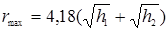
Therefore, at small distances the main factor enabling radar monitoring of flying birds is a tilt angle value that exceeds a certain criterion threshold rθ / 2. At larger distances the tilt angle can be decreased, although in this case the curvature of the Earth will have an impact. Both factors can be properly taken into account using a formula that yields the value of the minimum height (meters) depending on the distance (kilometers), this values being the root of sum-of-squares of (7) and (8):

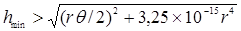(9 )

In (9) the first summand under the square root sign depends on the beam width, while the second summand does not. As the beam width decreases, the radar ability for detecting low-flying birds increases; this said, the bottom limit of the height can not be equal to zero, as it depends on the curvature of the Earth. Abshaev (1980) suggests a different formula for calculating the minimum height at which a target can be detected at normal refraction values:

h = r sin θ+βr²,

where r is the distance to the target, θ is the tilt angle and β=6×10^-5 km.

The second summand takes into account the difference between the radius of the Earth curvature and the beam trajectory under conditions of normal refraction. At normal refraction values, if the radar is located at sea level and the beam is 0,5⁰ , the minimum height at which birds can be detected is 400 m at the distance of 50 km, and 700 m at the distance of 100 km. In case the radar is located above seal level, these values are significantly lower. For instance, MRL-5 radar in Latrun (Israel) is located at 270 m above sea level. At normal refraction conditions, this radar is able to detect all the birds at the distance of 25 km at the horizon level (θ = 0⁰) even at a certain negative tilt angle. At distances of 50 km and 100 km, this radar can monitor birds flying at the heights of 100m and 400 m relative to the radar location level, respectively.

These calculations show that at lower heights the main factor restricting the range of radar vision is not the radar station potential, but rather the curvature of the Earth, the height of the radar location above sea level, openness of the horizon and the beam width. This means that the actual minimum height at which birds can be detected depends on the parameters of the underlying ground, in particular on its hilliness and the heights at which birds are flying. The Tables below present the maximum values for ranges of visions accessible by MRL-5 along various directions when birds are flying at the minimum height. In fact, these distances are different for different scanning directions and depend on the extent of “openness" of a particular direction for the radar beam. Table 2 presents dependencies of the distance of birds’ detection on their flying height, experimentally established by means of MRL-5 in Latrun (at zero tilt angle).

Table 2. Distances at which birds can be detected depending on their flying height.

4. Accuracy and resolution capacity of radar bird monitoring

Accuracy and resolution capacity of the radar while locating a single bird or a bird flock is determined by well-known dependencies characterizing radar location of a dispersed multiple target

(Battan, 1959). A highly important component of our computer-controlled station is the system of averaging over space and time that enables to isolate the target signal against the background noise. However, averaging over space and time leads to a certain expansion of the signal in comparison to the radar’s own signal. For this reason, one should take into account the parameters of the entire station rather than the radar itself. The algorithm and the design of the system for averaging over space and time is described in detail elsewhere (Battan, 1959); it is important to point out that its main parameters are: a) the number of averaged probing pulses while averaging over distances and b) the number of averaged scanning intervals while averaging over the angle . For the system to perform efficiently, the product of these coefficients has to obey the condition

> 50. If the amplification band of the radar receiver matches the frequency band of the probing signal, the accuracy and resolution capacity of the radar in bird monitoring can be calculated by the formula

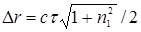(10 )

In the tangential direction, the accuracy and resolution capacity obey the expression

(11. )

In both (10) and (11), is the angle velocity of antenna rotation and is the scanning interval.

At small tilts, the magnitude of the spike is chosen to be equal to the beam width, so.

As can be seen from (10) and (11), neither the resolution capacity nor the accuracy regarding the detection distance depend on the distance to the target; at the tangential coordinate and height-wise, both the accuracy and the resolution capacity are proportional to the distance to the target.

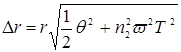
Height-wise, the accuracy and resolution capacity are calculated as

12

where is the value of a spike at the tilt angle.

We can now calculate the accuracy and the resolution capacity over the coordinates for the computer-controlled station based on MRL-5 meteordar. The parameters of the radar are the following: pulse duration

= 1 mcs, =4, = 18,

0,5⁰ p = 0,017 rad,

= 36⁰/s = 0,314 rad/s, = 2 ms.

The power of bird echo does not usually exceed 30 dBZ, with means, that the beam usually catches the echo within its center. Therefore, one can reliably assume that the width of the active segment of the beam able to detect a weak signal reflected from a bird does not exceed θ/2=0.25⁰=0.0085 rad. Thus for distances of 20 km and 50 km the resolution capacity required for separating bird echoes is, as regards the height and the tangential component, 200m and 400m, respectively. The resolution capacity distance-wise does not depend on distances and is 150 m.

5. The probability of bird detection at various distances from MRL5(Is) established experimentally

The method for assessing the probability of bird detection at various distances from MRL-5 (Is) is described elsewhere (Dinevich and Leshem, 2008). Tables 3 and 4 show some findings from the study relevant for a certain scanned area (Latrun, Israel, radar location at about 300 m above sea level).

Table 3. The probability of bird detection at various distances from the radar at night

(λ =10сm)

Table 4. The probability of bird detection at various distances from the radar in daylight

( λ =10сm)

In addition to Tables 3 and 4, we present below two ornithological charts of bird migration at night and in daylight (Fig. 2 and 3), as well as graphs of the mean height of the maximum bird concentration in daylight (autumn 2009) and at night (2010) (Fig.4) and in daylight (spring 2009) and at night (2010) (Fig.5).

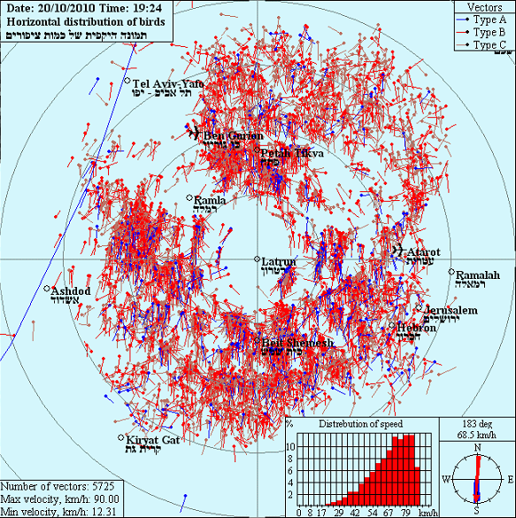
Fig. 2 shows a chart for the bird flow on October 20, 2010, at 19.24 p.m. within the radius of 40 km from the radar.

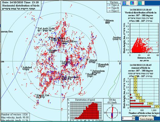
Fig.3 presents a sample of bird flow chart for October 14, 2010, in daylight (13.18 a.m.).

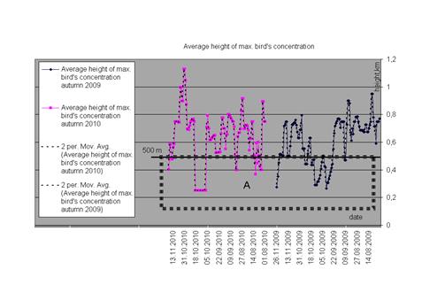
Fig.4. The mean height of the maximum bird concentrations in autumn in daylight (2009) and at nighttime (2010). In case the height falls within A zone, i.e. falls below 500m, the detection distance does not exceed 30 km.

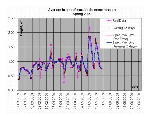
Fig.5. The mean height of the maximum bird concentrations in daylight (spring, 2009). In case the height falls below 400 m, the detection distance does not exceed 30 km.

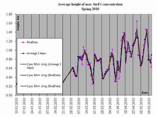
Fig. 6 ( Fig.4, 5 and 6), the distance at which birds can be detected, both in daylight and at night, is below 30 km).

Fig. 2 shows a chart for the bird flow on October 20, 2010, at 19.24 p.m. within the radius of 40 km from the radar. One can see 5725 vectors oriented from the south to the north, almost all of them colored red. Those are vectors of echoes from birds whose flight speed is variable, and flight direction deviates from a straight line by not more than 20%. There are a few blue-colored vectors of echoes from birds flying strictly along a straight line at permanent speed. Vectors of echoes from birds flying at highly variable speed and in frequently changing directions (absent in this case study) would be marked brown.

The graph below shows the speed spectrum of the vectors. The red arrow indicates the average flight direction for the total of the migrating birds. As can be seen in Table 1, situations like that are observed in the region in 35-52% of cases. The limitations are mostly accounted for by the flight heights and the orography of the surface (it is covered by hills at low heights).

Fig.3 presents a sample of bird flow chart for October 14, 2010, in daylight (13.18 a.m.). The notation is the same as that in Fig.2 The scan radius is 50 km, the number of vectors is 1836, the maximum flight speed is 90 kmh, the minimum flight speed is 12 kmh. In the right bottom part of the figure we see the speed distribution pattern (the red arrow within the circle stands for the average flight direction over the total of the birds); the blue vectors indicate the echo from birds flying along a straight direction at a constant speed. The red vectors mark the echo from bird flying at variable speed, with a deviation from the straight direction by not more that 20%. The right bottom part of the figure shows the distribution of the vectors over height (by 500m layers), and above it we see the projection of all the echoes within the scan area onto the vertical plane.

In the middle part of the figure we can see long strips of bird flock echoes (some as long as 90 km interrupted sometimes with gaps), as well as multiple echoes from small flocks and single birds. Flight pattern of this type is typical of the conditions of a developing convection.

Unlike night flights, daylight flights of migrating birds are most often shaped as strips oriented in parallel to the coast line. At heughts within A zone (below 400m, Fig.4, 5 and 6), the distance at which birds can be detected, both in daylight and at night, is below 30 km.

In autumn (Fig. 4), both in daylight and at night, the height of maximum bird concentration varies day to day, but does not have a distinct pattern for a specific month. In spring the picture is entirely different – the height of maximum bird concentration, both in daylight and at night, increases month by month. The higher birds fly, the larger the distance at which they can be detected.

As it was mentioned above, the analysis of the charts and the graphs shows that, the parameters of the terrain and flight heights being taken into account, not less than 35-52% of night-flying birds can be detected at the distance of 40 km. At the distance of up to 60 km, MRL5 (Is) is able to detect about 20% of night-flying birds. However, this is true in case the flying height does no exceed 400 m. The daytime-flying bird species are usually bigger than night ones (among them storks, pelicans, eagles, honey buzzard and the like). The SCS of these species and, consequently, their echoes are larger than those of night-flying birds. While flying, these larger birds often take advantage of convective atmospheric flows that form due to inhomogeneity of the ground surface, as well as to the upland-valley breeze processes. These birds often form strips as long as 90-100 km. The analysis of our daytime observations (Table 4) shows that MRl5(Is) is able to detect not less than 80% of migrating birds at the distance of up to 30 km, which is close to the number of birds detected at night. As to the daytime-flying birds, MRL5(Is) is able to see up to 60% of them at the distances of up to 60 km. The detection distance and the probability of achieving a larger detection rate well correlates with the flight height and the degree to which the ground surface the birds fly over is open for the radar beam. In favorable conditions, MRL5(Is) is able to detect up to 83 % of all flying birds within the maximum scan radius.

It is clear that there are significant variations in the system’s ability to detect all the birds within the scan area of 60-km radius. The analysis described above enables to determine several factors that may account for these differences:

• in some cases, birds (or part of birds) fly beneath the radar beam level;
• part of the migrating birds crossing Central Israel fly over the Jordan Valley which is situated much below the level accessible by means of MRL5(Is). The lower part of the Jordan Valley near the Dead Sea is located 500 m below sea level, i.e. about 800 m below the height of the radar location;
• the character of the terrain lying beneath the route of migrating birds is an important factor, since those routes often go along valleys located between high hills and thus unreachable for a radar;
• the completeness of the data depends on the management of systematic observations, including uninterrupted schedule and interpolation for periods between scans.

5. On the issue of number of birds flying over Central Israel in autumn and in spring.

In view of considerations presented above, the quantitative assessment of absolute numbers of birds flying over Israel should be regarded as approximate only. However, taking into account the vast corpus of seasonal data, we believe that relative characteristics (i.e. data comparison over lengthy periods of time) can be representative for various other assessments (see graphs in Fig.7 (a, b, c) and Fig.8 (a, b, c).

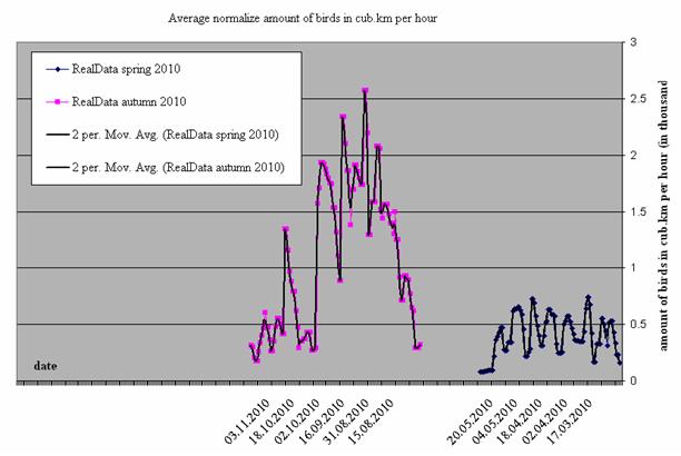
Fig. 7 (a) presents the number of birds that flew over Central Israel at night in autumn and spring in 2010.

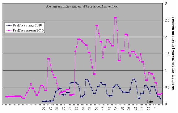
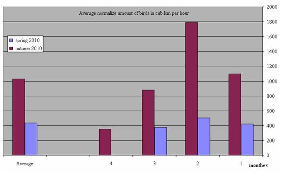
Fig. 7 (a) presents the number of birds that flew over Central Israel at night in autumn and spring in 2010.

Fig. 7 (b, c) clearly shows that the number of birds is larger in autumn than in spring. Along the X-axis we see the 91 spring observation days (from March 1st to May 31st) and the 120 autumn observation days (from August 1st to November 30th). Fig. 7(c) shows the number of birds for each months and the calculated mean bird number values for both seasons.

As can be seen from Fig. 7 and 8 (a,b) both in daylight and at night significantly more birds fly over Israel on their way from Europe to Africa, than in the opposite direction in spring (the autumn/spring ratio is 1:1.5 for daylight and 1:2.5 for night flights).

We suggest the following reason to explain these differences. Part of the birds die during wintering in Africa, and new progeny is not born there. During summer months “at home” in Europe new nestlings are born, raised, taught to fly and thus prepared for the migration flight. In short, birds fly to Africa with enlarged families and return having suffered severe natural loss in population. Bird species migrating in daylight have fewer nestlings than bird species flying at night.

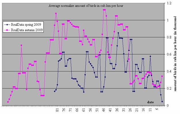
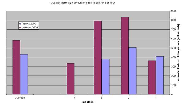
Fig.8 (a, b) shows the same parameters for spring (2009).

Our findings may enable to approximately assess the percentage of bird loss during wintering and the percentage of bird population increase during their stay in the “home environment” in Europe.

A long-term study and a massive database are needed in order to conclude if these conclusions are of regional relevance only and if we may speak of a steady year-to-year pattern.

7. On the accuracy of establishing the directions of bird flights in autumn and spring.

Fig. 9, 10 and 11 present graphs for distribution in flight directions of birds in different situations (day, night, autumn, spring)

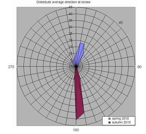
Fig.9 presents the distribution of flight directions at night (autumn and spring, 2010).

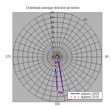
Fig. 10. Distribution of flight directions in autumn (80% of migrating birds) in daylight (2009) and at night (2010).

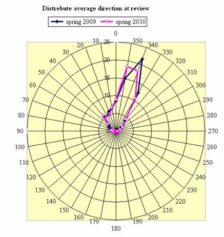
Fig. 11. Distribution of flight directions in spring (80% of migrating birds) in daylight (2009) and at night (2010).

The direction of spring flights is opposite to that in autumn. In daytime birds mostly fly in strip-shaped or small groups, while at night we see large bird flocks.

By way of example, Fig.9 presents the distribution of flight directions at night (autumn and spring, 2010). Fig. 10 and 11 show the spectra of these directions for 80% of migrating birds, both in daylight and at night, in autumn and in spring. For autumn, all the spectra of both daylight night flight directions fall within the range of 180-190°, and for autumn – within the range of 30- 320°.

In order to explain these seasonal differences in flight direction spectra for birds on intercontinental flights, further research is needed.

Conclusions

• Under conditions of normal refraction at distances of 5-25 km, MRL-5(Is) is able to detect all the birds (undisguised by hills) at the horizon level (q = 00); in some directions, the birds can be detected even at a certain negative angle.
• At low heights, the main factor restricting the distance of radar bird monitoring is not the potential of MRL-5, but rather a set of other factors such as the curvature of the Earth, the height of the radar location (above sea level), the openness of the horizon for the radar beam and the beam width. A bird as big as a stork flying at over 400 m above sea level (i.e. at 100 m relative to the radar location height) reflects an echo strong enough to be detected by the radar at the distance of 90 km.
• In daylight, at the distance up to 60 km from the radar, under conditions of the open horizon, the station detects 56-83% of migrating birds flying at the height of over 400 m above sea level (i.e. at 100 m relative to the radar location height). The undetectable birds either fly below the beam level or are disguised by hills.
• At night, at the distance up to 30 km from the radar, the station detects 74-89% of migrating birds flying at the height of over 250 m above sea level (i.e. only at 150 m relative to the radar location height).
• At distances of 20 km and 50 km, the resolution capacity of the station (i.e. detecting separated echoes of two or more birds flying at distance from each other) is 200m and 500 m, respectively; regarding the height and the tangential component; distance-wise, the capacity is 150 m regardless the distance to the target.
• Systematic observations of seasonal bird migration in daylight and at night conducted during two autumn seasons and two spring seasons showed that the number of birds flying via Israel from Africa to Europe is significantly lower in spring than in autumn. For daylight, this proportion is about 1:1.5, and for night time is about 1:2.5. The most likely reason to account for this difference is the fact that part of the birds die in Africa during winter and new progeny is not born. On the way back from Europe to Africa birds fly together with the new progeny. These findings enable to approximately assess the percentage of bird loss during wintering and the percentage of bird population increase during their stay in the “home environment” in Europe. A long-term study and a massive database are needed in order to conclude if these conclusions are of regional relevance only and if we may speak of a steady year-to-year pattern.
• Flight directions in autumn practically do not differ from those in spring, although in autumn the dispersion (spectrum) of these directions is much narrower than in spring. Further studies could cast light on the reasons underlying this phenomenon. On the potential development of the system.
• On the basis of a number of studies, including those by the authors of this paper, it has been shown that fluctuation parameters of radar echo can be effectively used to distinguish signals reflected from single-flying birds at high accuracy. A sound representation of the fluctuation gives a good understanding of the bird’s orientation in space and the wing-flapping pattern. Using the Radar Equation one can measure the SCS of the bird and thus determine its size at a certain degree of accuracy. These characteristics together with the pattern of a bird’s movement give some indication concerning the bird’s species. By measuring the level of radar reflectivity within each scanning area and knowing the species and SCS of the birds, we can approximately assess their numbers and spatial concentration.
• The algorithm for bird echo isolation developed for MRL5(Is) should be adapted for Doppler radars. This will enable both to significantly reduce the time needed for data update and to increase the accuracy. The issues related to the development of the adapted algorithm and the corresponding software is a matter of further research aimed at advancement of MRL5(Is) that goes beyond the scope of this paper. We hope that prospected establishing the Center for Bird Migration Monitoring in Latrun (Israel) will open new perspectives for achieving this goal.
• In view of the specific orographic characteristics of the territory of Israel, at least six radar stations of MRL-5(Is) type should be installed in order to ensure detection of at least 80% of migrating birds. Two of these stations should be used for observations over the lower parts of the Jordan Valley.

Acknowledgements

The authors express their gratitude to the Department of Science of the Ministry of Defense of the State of Israel for the financial support of the project, to the administration of Tel Aviv University for their continuous interest in the project, as well their deep thanks to several people for the important contribution: to Alexander Kapitannikov and Oleg Sikora who assisted in designing components of the software; to Vladimir Dinevich who helped to install the radar, to Valery Garanin and Dmitry Shtivelman who provided the technical maintenance of the radar, and Prof. Arcady Shupijatcky for his decades-long friendship and constructive work on this paper. The authors wish also to specially acknowledge the contribution made by the late Prof. Lev Kaplan.

Appendix

The terminology and notification.

1) Receiver sensitivity Pn is the minimum power of a radar echo at the receiver entry that enables to obtain a nominal (set) value of the output voltage (at the given signal/noise ratio) that enables to steadily fix the signal against noise. Receiver sensitivity is usually measured in watts (W) and its values are within the range of 10-12 to 10-14 W.

2) The radar beam θ characterizes the directional parameters of the radar antenna that affect the accuracy of determining the target coordinates. The shape and the width of the beam may differ depending on the purpose of the station. The beam width of half power is the angle between directions in which the radiated power is 50% of the maximum power radiated along the beam’s axis. The shape and the width of the beam depend on the type and dimensions of the antenna, as well as on the wavelength λ.

3) Resolution capacity – the resolution capacity may be related either to the distance or the coordinates. Resolution over distance (rmin) is defined as the minimum distance between targets that are located along the same direction relative to the radar, at which those targets can be perceived by the radar as separate ones. In case the distance between the targets is below this minimum distance, the echoes of the targets merge on the radar screen. The resolution capacity over distance depends on the technical parameters of the equipment and the duration of the pulse within this space h=c·τ, where c is the light speed and τ is the pulse duration (in sec).

Resolution capacity over coordinates is defined as the minimum angular distance between targets located at the same distance, at which those targets can be perceived by the radar as separate ones. Resolution capacity over coordinates depends primarily on the radar beam width within the corresponding plane, as well as on the resolution capacity of the indicating equipment.

4) The radar distance – radiowaves of length within the centimeter range propagate in the atmosphere within the line-of-sight, their trajectories being curvilinear rather than straight (the trajectory of radiowave propagation is called a beam). This happens due to atmospheric refraction caused by the dielectric inhomogeneiety of the atmosphere.

5) The radar equation for single targets – the radar equation relates the power of the echo with the technical parameters of the radar station, with the reflective properties of a target and the distance to it, as well as the conditions of radiowaves propagation on their way to the target.

6) Scattering cross-section of a bird – the reflective ability of a bird is determined by the dielectric properties, the shape and the dimensions of the bird’s body. It also depends on the length and the polarization of the incident wave.

2. Abshayev M., Kaplan L., Kapitannikov A., 1984. Form reflection of meteorologic targets at the primary processing of the meteorologic radar signal. Transactions of VGI, Bd 55 (in Russian).

3. Battan, L., 1959. “Radar meteorology”, 161 pp. Univ. of Chicago Press, Chicago, Illinois.

4. Chernikov A., Schupijatsky A., 1967. Polarization characteristics of radar clear sky echoes. Transactions of USSR academy of sciences, atmosphere and ocean physics, V.3, N2, 136-143. (in Russian)

5. Chernikov A., 1979. Radar clear sky echoes. Leningrad, Hydrometeoizdat, 3-40. (in Russian).

6. Dinevich L., Kapitalchuk I., Schupjatsky A., 1994. Use of the polarization selection of radar signals for remote sounding of clouds and precipitation. 34th Israel Annual conference on Aerospace sscience, 273-277.

7. Dinevich L., Leshem I., Gal A., Garanin V., Kapitannikov A., 2000. Study of birds migration by means of the MRL-5 radar. J. Scientific Israel –Technological Advantages. Vol. 4.

8. Dinevich L., Leshem Y., Sikora O., 2001. RADAR OBSERVATIONS ANALYSIS OF SEASON BIRD MIGRATION IN ISRAEL AT NIGHT (Based on data of radar photo registration obtained in 1998-2000), J. Scientific Israel –Technological Advantages, Vol. 3, 2001, No. 1-2.

9. Dinevich L., Matsyura A., Leshem Y., 2003. Temporal characteristics of night bird migration above Central Israel radar study. ACTA ORNITOLOGICA vol. 38 (2). P. 103-110.

10. Dinevich L., Leshem Y., Pinsky M., Sterkin A., 2004. Detecting Birds and Estimating their Velocity Vectors by Means of MRL-5 Meteorological Radar. J. The RING 26, (2): 35-53.

11. Dinevich L., Leshem Y., Matsyura A., 2005. Some Characteristics of Nocturnal Bird Migration in Israel Accordding to Radar Monitoring. The Ring 27 (2). P. 197-213.

12. Dinevich L., Leshem Y., 2007. ALGORITHMIC SYSTEM FOR IDENTIFYING BIRD RADIO-ECHO AND PLOTTING RADAR ORNITHOLOGICAL CHARTS. J. The RING 29, (1-2): 3-39.

13. Dinevich L., Leshem Y., 2008. Isolation of radar echo from migrating birds and plotting ornithological charts on th basis of data obtained on the basis of MRL-5. Uspekhi sovremennoi radioelectroniki, # 3, 2008. 48-68 (in Russian)..

14. Dinevich, L. 2009. Radar Monitoring of Bird Migration. Tel Aviv University. November, 2009. pp. 1-173

15. Doviak, R., Zrnic, D., 1984. Doppler Radar and Weather Observation. Akademic Press Inc., 512pp.

16. Ganja I., Zubkov M., Kotjazi M., 1991. Radar ornithology, Stiinza, 123-145. (in Russian).

17. Gauthreaux, S. A. and C. G. Belser (2003). "Radar ornithology and biological conservation." Auk 120(2): 266-277.

18. Glover K., Hardy K., 1966. Dot angels: insects and birds.-In: Proc. 12th Weather Radar Conf., Amer. Met. Soc., Boston, 1966, p. 264-268.

19. Houghton E, 1964. Detection, recognition and identification of birds on radar. In: World conf. Radio Met., Amer. Met. Soc., Boston, 14-21.

20. Hajovsky R., Deam A., La Grone A., 1966. Radar reflections from insects in the lower atmosphere.-IEEE Trans. On Antennas and Propagation, vol.14, pp224-227.

21. Konrad T. G. Randall D., Simultaneous probing of the atmosphere by radar and meteorological sensors.- In: Proc. 12 th Weather Radar Conf. Amer. Met. Soc., Boston, 1966, p. 300-305.

22. Konrad T. G. Hicks J. J. Tracking of known bird species by radar.-In: Proc. 12 th Weather Radar Conf. Amer. Met. Soc., Boston, 1966, p. 259-263.

23. Leshem Y., Dinevich L., Matsyura A., 2003. Studying Raptor Migration by a network of Radar across Israel and Developing a Real Time Warming System for Flight Safety through the Internet. 6-th WORLD CONFERENCE ON BIRDS OF PREY AND OWLS, Budapesht, Hungary, 18-23 May, 2003

24. Richardson W. J. and T. West, 2005. Serious Birdstrike Accidents to U. K. Military Aircraft, 1923 to 2004: Numbers and Circumstances. IBSC 27th Meeting, Athens, Hellas, 23-27 May 2005. p. 5.

25. Rinehart R. F. Radar detection of Birds in New Mexico - Preperint, Illinois State Water Survey, 1966, 6p.

26. Stepanenko V., 1973. Radiolocation and meteorology. Gidrometeoizdat, Leningrad (in Russian).

27. Shupijatcky A., 1959. Radar dispersion of nonspherical particles. Transaction of CAO, vol.30, pp.39-52 (in Russian).

28. Zavirucha V., Saricev V., Stepanenko V, Shepkin U., 1977. Study of the dispersion characteristics of the meteorological and ornitological objects in echo-free cameras Proc. Main Geophysic Observatory, #395, с. 40 –45 (in Russian)

29. Zrnic, D. S. and A. V. Ryzhkov (1998). "Observations of insects and birds with a polarimetric radar." Ieee Transactions on Geoscience and Remote Sensing 36(2): 661-668.

30. Shestakova, G., 1971. The structure of bird wings and the mechanics of bird flight. Moscow, 180 p. (in Russian).