Accelerometer by is compensation is designed to measure linear acceleration of moving objects. Information of linear acceleration is required for the purposes of motion control the object, for the purposes of orientation and navigation. Accelerometers are commonly used to measure the deviations from the vertical (horizontal), measuring the motion parameters, measurements of vibration parameters. Compensatory accelerometers are sufficiently precise measuring instruments  (sensors of inertia), manufactured by specialized the companies industry.

This article discusses the development of mathematical model and computing imitation of the accelerometer based on this model. The sensor linear acceleration a uniaxial is accelerometer, it is considered by compensating for pendulum-type, sensing element of  with elastic the suspension, a capacitive the sensor displacement and the sensor is magnetic-type feedback . The sensing element is made of monocrystalline silicon. Design features of accelerometer and schematic is presented in article [1].

The design of the accelerometer sensor element comprises: the permanent magnet; a tip of a soft magnetic material;  magnetic circuit; coils; an arm of fastening of the coil; a temperature sensor;  crystal element of the pendulum; optical glass; a collar connecting the magnetic system.

The article [2] in addition to the materials [1] briefly a block diagram of an the accelerometer, reflecting its dynamic mathematical model. On the block diagram shows all the functional elements of the accelerometer in the form of transfer functions: Kche - transfer coefficient of the sensor element (SE); Wpu - transfer function of the motion node (is the pendulum); Kpp - coefficient of  transfer transducer of displacement; Wku - transfer function of the device of correction; Wn - the transfer function the load; Kos - the ratio of transmission of feedback element.

The total transfer function is calculated according to the block diagram of [2]:

.                                                      (1)

For the calculation of the mathematical model of W (s) based on the software environment Matlab was drawn up program, consisting of a controlling part and sub-functions. When calculating W (s) used  the design parameters of the accelerometer and the parameters of the electrical circuit diagram [1]. The control part of the program is presented in the form of the next text.

[Amax, am, bm, cm, lcm, h, Uo, Ku, C] = input () - the task of initial data;

[Kche, Se, Sv, So, m] = che (lcm, am, bm, cm) - calculation of gain of sensor element;

[Ja, Kdm, Wpu] = PU (am, bm, cm, m, h, lcm) - calculation of the transfer function of the motion node;

[Co, Kpp] = dpp (h, lcm, Uo, am, Se, So) - calculation of the displacement sensor coefficient;

[Km, Rm] = DM (lcm) - calculation of the transfer coefficient the sensor of feedback;

[Wky, We, Rn] = electr1 (amax, Rm, Kche, Km, C, Uo, h) - calculation of the transfer function the devices of correction and electron unit;

[Wz] = Wpoln (Kche, Ku, Wpu, Kpp, We, Rn, Km) - calculation the total of the transfer function of sensor.

The element of pendulum of accelerometer and the device of  motion. Based on the known parameters of the accelerometer structure, calculated the main parameters of the pendulum element: mass and moment of inertia of the pendulum, the rigidity of the elastic suspension; damping factor. In the end, for the pendulum element is calculated transmission coefficient of the sensor element - Kche and the transfer function of the motion node - Wpu.

Transfer Ratio  the sensor element - Kche calculated as follows:

KЧЭ =m∙ lЦМ,                                                                   (2)

where m - mass of the pendulum; lcm - the distance from the rotation axis to the center of mass.

Calculation of the moving part SE pendulum consists in finding parameters: of mass,  of moment of inertia and of damping coefficient.

To measure the linear acceleration in range of ±10g, where g - acceleration of free fall, for  pendulum  of tipical the size is calculated: the  mass of pendulum, the coefficient of transfer and the moment of inertia, which amounted to following values: m=2,0337∙10-4 kg; Kche=8,34∙10-7; Ja=1,31∙10-8 - the moment of inertia of the pendulum with respect to the rocking axis. For the motion node pendulum is calculated: damping coefficient: Kdm=5,63∙10-5 H; rigidity elastic suspension: Gy=0.0018 N ∙ m / rad.

The final stage of the calculation of the motion node is to calculate its transfer function Wpu.

.                                                     (3)

For the previously computed parameters Ja, Kdm, GU, Wpu transfer function is defined as:

.                                     (4)

The transfer coefficient of primary sensor displacement. In this accelerometer is applied capacitive pickup scheme of signal, which implies the existence of capacitors of the sensor primary converter, the Capacity  of which vary depending on the deflection of the movable member.

Capacity flat capacitor is determined by the formula: (5)

,                                                                    (5)

where εo, ε - absolute and relative permittivity of medium; S - working area of the capacitor plates, m2; h0 - the distance between the plates (gap), m.

The capacitor plates is a figure, of complicated configuration repeating the of crystal element, but without holes. Calculating all the electrode area we get: S=3,5146∙10-5 m2.

In this case, a capacitance dependent on the distance between the electrodes. The formula shows that this dependence is hyperbolic, so circuits using parallel-plate capacitor is expedient to operate with small gaps that provides a combination of linearity characteristics with high sensitivity. Furthermore, to ensure the linearity of the converter circuit using the differential measurement of two capacitor  - the bottom and top.

As a result, calculation for formula capacity flat capacitor (5), was: Co = 1,8348 ∙ 10-11 F.

The dependence of the upper and lower tanks of the plate movement is determined by the formulas:

where d=lcm ∙ α - movement of the plate depending on the angle of deflection. The dependence of the upper and lower ca pacity for the plate movement is determined by the formulas:

, ,                                                         (6)

where d = lcm ∙ α - movement of the plate depending on the angle of deflection.

The  function is convert of differential capacitive sensor represented as a ratio of the difference shoulders to their sum. Algorithm of transform the capacitive sensor in the output voltage is as follows:

UПП=UОП(C1–C2)/ (C1+C2),                                                   (7)

where Uop - a reference voltage; C1, C2 - variable capacity of angle sensor.

On figure 1 shows the complete block diagram of the electronic unit, compiled on the basis of the principal electric accelerometer scheme [1].

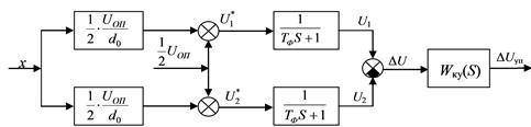
Figure 1 - Block diagram of the electronic unit

(X - movement of motion node; d0 - gap between the movable plate and the lining)

This scheme allows in the capacitive sensor C1 and C2 make the transformation in U1* and U2* voltage and then by filtering, transforming them into the U1 and U2. Further, by calculating the voltage difference: ΔU = U1 - U2 obtained by the algorithm of the primary motion transducer in accordance with the formula (7). The circuit comprises a correction unit with filters.

The voltage difference between the channels, forming the of differential measurement algorithm.

.                                                 (8)

In case of equal resistors R1 = R2 obtained the algorithm of the  sensor of primary transformation in accordance with the formula (9).

.                                               (9)

where d0 - the gap between the fixed and movable plates; x - moving the movable plate (crystalline element).

Thus, coefficient primary transducer according to the movement of the plate is determined by the formula:

KПП = U­ОП / d0.                                                                      (10)

Substituting the original data into the formula (10) we get: Kpp = 2,56 ∙ 105 V / m.

Transfer function of correcting device and electronic unit. Given the passive low-pass filters the PWM converter and the RC chain concept [1], transfer function the correcting device has the form (11).

.                                                (11)

To calculate the load resistance, the coefficient of the primary transducer (Kpp) and transfer functions the correcting device and the whole of the electronic unit (We)  has been developed program-function:

[Wky, We, Rn] = electr1 (amax, Rm, Kche, Km, C, Uo, h).

When calculating the transfer function the device of correction used data as: k1=R8/R6; k2=(R3+R5)/R4; T2=C3∙R8; Tf∙Rf=CF; r1= Cky∙(Rky+R4); r2=CkuRku. As a result, Wky received as follows:

.                                                 (12)

The transfer function of the electronic unit comprises a unit with a coefficient of primary transducer (Kpp), the transfer function Wky and link load: W1 = 1 / (Rn + Rm). As a result calculation the load resistance value was: Rn = 313,3 ohm, and the impedance of the two coils: Rm = 64,5 Ohm. As a result, We got the following form:

.                                                 (13)

The ratio transmission of the torque sensor. The compensation instruments found widespread use as a reverse converter of magneto-electric sensor. The main positive effects of the magnetoelectric sensor are: linearity, the ability to compensate for temperature errors and compared with other converters, a large value of developed force.

When calculating the torque sensor is first calculates the magnetic flux density in the gap of the pendulum. The next stage is calculated the number and turns of the coil wire length. Based on the calculated total length of wire  calculated resistance of coils. In this case, the calculation was carried out using a specially designed program-function: function [Kdm, Rm] = DM (lcm). As a result of the calculation was obtained torque sensor transfer coefficient: Kdm=2∙Bp∙lpr∙lcm=0,0051, and the total impedance of the two coils: Rm = 64,5 Ohm.

The full  transfer function of accelerometer. In begin section of construction of a mathematical model of the accelerometer was formed full expression of the accelerometer transfer function, which is represented by formula (1). Further, all elements, included in the transfer function expression were calculated. When calculating the transfer function of the electronic unit has been used: We = Kpp ∙ Wky, uniting transducer displacement and correcting device.

As a result, based on the expression of full transfer function of an accelerometer (1) to calculate the total transfer function of the accelerometer in numerical form was obtained:

                  .                                     (14)

Transmission ratio of accelerometer in accordance with the transfer function is obtained: K=dcgain(Wz) = 0,0508.

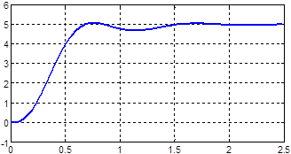
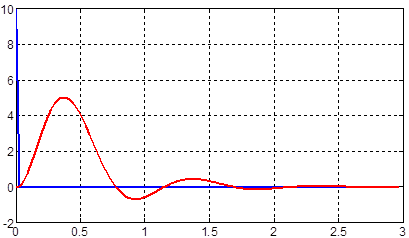
Checking of mathematical model of accelerometer was held by a Matlab simulation software environment. Simulated the action input as a linear acceleration was at the border of the working range (in this case +10g). In this case, when applying of linear acceleration for input signal a 10g at the output was obtained with an adequate transition process, which is  set the value of 5V (see. Figure 2).

 ∙10-3 с

Figure 2 - The process of transition at the output of the accelerometer

This confirms the correctness of developed mathematical model: by the maximum input acceleration signal for accelerometer is working out in the  maximum output voltage.

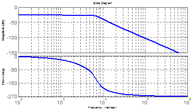
The next stage of testing a mathematical model DLU was sent to study the amplitude-frequency characteristics (AFC). By using Matlab function bode() was built logarithmic: amplitude-frequency and phase-frequency  response. These characteristics are shown in Figure 3.

 lg(ω) rad/с

Figure 3 - The amplitude-frequency and phase response of the accelerometer

The resulting theoretical AFC and phase response also confirms the correctness of the mathematical model of the accelerometer.

Bandwidth is calculated in downturn from 3 dB from the initial level. In according to the schedule, the bandwidth was about 3.6 decades or 3981 rad / s, ie, 633.6 Hz. The alleged characteristics of the accelerometer to 10g range, according to the developer information [1], was guaranteed bandwidth of 100 Hz. Thus, by proper selection of device of correction and it settings in a straight chain of accelerometer, able to improve its performance (increased bandwidth).

Imitation tests the accelerometer

Test of the accelerometer by of sinusoidal imitation. The computational experiment was performed by simulations in sinusoidal mode of input signal [3]. For the tests was used previously developed mathematical model of the accelerometer, and by role of vibration device performs sinusoidal source in the form of an electronic unit or program in Matlab environment.

For the experimental study of the accelerometer in sinusoidal mode has been developed management simulation program and subprogram-function AX_exp (). The control program is as follows:

Wz = tf ([0.03135], [3.92e-12 2.996e-8 2.4e-4 0.6169]) - transfer function of DLU

AX_exp (Wz) - experimental AFC

Sub-function is defined by the following text:

function AX_exp (Wz) - experimental AFC;

t = [0: 1e-4: 100 1e-4] - array of timestamps;

k = 1: = 51 km - number of AFC tests;

w = [0: 10: 8000] ' - frequency range, rad / s;

for k = 1: length (w) a (k) = 0; end - input of initial array of amplitudes;

for k = 1: length (w) - looping of through the entire frequency range;

u = 10 * sin (w (k) * t) - the input sinusoidal signal with an amplitude of 10 m / s2;

h = lsim (Wz, u, t) - obtain a response to the a sinusoidal impact of;

for i = 1: length (t) if a (k) <h (i) a (k) = h (i) - computation of the amplitude at the output of the DLU; end; end; end;

figure (2); plot (t, h, 'k', 'LineWidth', 2.5), grid - schedule on output DLU;

figure (3); plot (log10 (w), 20 * log10 (a), 'k', 'LineWidth', 2.5), grid - graph logariphmic AFC.

In this study a sinusoidal input signal of simulated in the intended frequency band (for accelerometer is from 0 to 8000 rad / s or to 1273 Hz). In is experiment was recorded sinusoidal sensor output signal in response to the input action. Next was measure the output amplitude of the signal, and as a result was built the graph of logarithmic amplitude-frequency characteristic of the sensor, which is shown in Figure 4.

   lg(w)

Figure 4 - The frequency characteristic of the sensor resulting from the experiment

The vertical axis represents the amplitude of oscillation of the sensor output in decibels, and a horizontal axis -  angular frequency in decades.

Bandwidth is calculated by of downturn AFC in 3 dB from the initial level. In  study the graph that the frequency axis gives about 3.6 decades or 3981 rad / s, i.e. 633.6 Hz.

This experiment studies the frequency response of the accelerometer in mode sinusoidal influences. Was confirmed its performance, stated on the passport  of values (obtained sufficient bandwidth).

Tests of the accelerometer in pulse mode. To investigate the effects for accelerometer of pulse input signals mode in the Matlab simulation was used program-function [h, dt] = pulse1 (Wz) [3].

The experiment was performed at pulse input impact of acceleration on the accelerometer. In the program as a test object was used  the transfer function of the accelerometer - Wz. Was imitation a short pulse of duration dt = 3 ∙ 10-5 s. Reaction of accelerometer  to action of pulse input is shown in Figure 5.

Imitation of surge was with an intensity of 10 m / s2 (just over 1g, where g - acceleration of gravity) and a duration of 3 • 10-5 with. When pulsed action besides research response of accelerometer was analyzed amplitude-frequency and phase-frequency response (APFC) sensor - W (jω).

·10-3 с.

Figure 5 - System processes reaction DLU with pulse action

We used the classic formula, based on the reaction to impulse action:

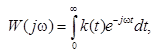                                                      (15)

where k (t) - impulse response function; ω - angular frequency.

To calculate the frequency response used the known relationship A (ω) = | W (jω) |. On the basis of (15), to calculate an approximate value for the discrete values of the frequency response is given by [4].

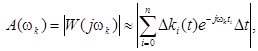                                        (16)

where ti - time interval; Δki - the value of the impulse response function at time interval; Δt - sampling interval of time; ωk - the discrete frequency.

The corresponding program for the calculation of the frequency response according to the formula (16) is shown in the following fragment.

Wz = tf ([0.0627], [3.92e-012 2.996e-008 0.0002414 0.6169]);% PF DLU

[H, dt] = pulse1 (Wz); % Response to impulse action

[F] = acx (h, dt); % Detection response.

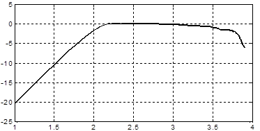
Figure 6 shows the frequency response graph for a process that appears at the output of DLU.

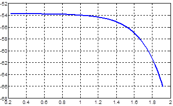lg(w)

Figure 6 - Schedule AFC DLU output process with pulsed action

From the graph it is easy to determine that the spectrum of the ACK process cutoff frequency is about 1.75 decades or 63 rad / s, i.e. 10 Hz (at of decline of logariphmic characteristic from the initial level of 3 dB).

For this linear acceleration sensor, according to a study by the impulse response, obtained fairly of low bandwidth - only 10 Hz. However, the in passport bandwidth the of sensor has a of 70 Hz. Earlier tests DLU  by mathematical model and on the basis of experiment  by the action sinusoidal signal  in the frequency range up to 5000 Hz, gave fairly acceptable results (bandwidth frequency DLU was  630 Hz).

Errors of the accelerometer

The main errors of the accelerometer are: deviation of the slope of the static characteristic (changing the scale factor) from nominal value; the nonlinearity static characteristic; the zero signal of accelerometer; error from of cross-acceleration; error from temperature [5].

To study the of errors of accelerometer was developed a control program, and the program functions in Matlab environment:

[Wz, n, ta, D, dUe, dUn, Amax, ar, Ap] = inp1 () - initial data input;

[K, Dk, sigmK] = krutizna (Wz, m, ta, D, dUe, dUn) - changing the scale factor of the accelerometer;

[Uom, sigmZ, Du] = zero0 (Wz, K, m, ta, D, dUe, dUn) - the zero signal of accelerometer;

[H1, H2, sigm1, sigm2] = noline (Wz, K, Uom, m, D, dUe, dUn) - the nonlinearity static characteristic of the accelerometer;

[dUp] = perekrest (ar, Ap) - error from the cross-acceleration;

[Dt] = summa (K, Dk, Uom, Amax, H1, H2) - error from temperature;

[Delt] = summa (K, Dk, Uom, Amax, H1, H2) - the total error.

When calculating errors were obtained the following results:

dK = 0,125% - error of the slope of the static characteristic;

dUo = 0,055% - the zero signal error (offset of zero);

dUn = 7,17% - error of non-linearity of the accelerometer;

dUp = 0,64% - error of cross-acceleration;

dUkt = 19,6% - temperature error.

Comparison of results for the errors of the accelerometer, obtained by simulations with the published data for a range of ±10g, suggests the adequacy of the experimental values (obtained similar data see. Table 2).

Table 2 - Comparative characteristics  of the results of the experiment and

Conclusions

According to the results of the experiment the most significant errors the deviation scaling factor from the norm - 0.125% and the temperature error - 19.6%.

It should be noted that the zero signal can be partly reduced by calibrating static characteristic of accelerometer immediately after its installation on a base surface of the movable object.

You should also bear in mind that the temperature error, mainly compensated algorithmically on the testimony of temperature sensors, mounted directly on of the pendulum of accelerometer. The temperature error was compensate  by algorithmic to a value of not more than 0.068%, which is acceptable for use the accelerometer as a measuring device.

Total accelerometer error (without taking into account the dynamic error, stationary random noise and errors arising from the impact of external factors and temperature error) is obtained in the form of: Δx = 7,35%. In the passport data the general error of the accelerometer has values - 1,554 %. High overall error (7.35%) was obtained by taking into account all factors affecting the operation of the accelerometer, which is not always the case in real-world conditions.

The main scientific and practical results in the article:

1. Was conducted a reasoned analysis of the objectives of the project in accordance with modern trends in the development of engineering and technology;

2. Developed the functional and structural schemes at level the elements and blocks;

3. By analysis of the physical model compensating the of accelerometer was made  calculation a blocks of the circuit and the full mathematical model of the accelerometer using the physico-mathematical formulas;

4. Was conducted  simulation of the accelerometer based on a mathematical model and conducted  analyzed the results using computer-aided design based standard packages and  software self-developed;

5. Was obtained typical the process of simulation and parameters of the accelerometer;

6. Was revealed shortcomings the of accelerometer and it was given recommendations to improve its performance;

7. Was given the objective assessment of the theoretical and experimental results, and was given a reasonable conclusion on the work done.

Carrying out the experiment of the accelerometer based on calculation of the mathematical model is quite justified and allows you to mark a high possibility of mathematical modeling and  testing by imitation.

2. Volkov VL, Karimov RN. Mathematical modeling the monitoring system of the parameters serial inertia sensors. / -M :. Academy of Natural Sciences. "International Journal of Applied and Basic Research", 2016, number 5, part 3, p. 365-370.

3. Volkov VL, Karimov RN Modeling the monitoring system serial sensors. / -Penza: Articles XVI VNTK. Aerospace equipment, high technology and innovation - 2015, Perm National Research Polytechnic Institute. 2015, page 27 -. 31.

4. Volkov, VL Mathematical modeling in instrument systems: Proc. Benefit / VL Volkov, NV Jidkova. NGTU them. RE Alekseeva. -N.Novgorod: 2014. - 147 p.

5. Evstifeev MI, Stepanov OA, Chelpanov IB. Tests micromechanical devices: Proc. Benefit / - St. Petersburg: Publishing JSC "Concern" Central Research Institute "Elektropribor". 2013 - 210 p.