Introduction

In the last decade mathematical models with linear and nonlinear long-range dependence have been widely adopted for the statistical description of the processes and structures in various complex systems with scale-invariant properties. Relevant properties have been observed, for example, in the primary DNA [Peng et al., 1994] and protein [Yu et al., 2003] structure, physiological rhythms [Ivanov et al., 1996], [Ivanov et al., 1999] and many other data records from complex systems. It has been shown that scale-invariant models can be used efficiently, for example, as diagnostic tools in biomedical research [Huikuri et al., 2003], [Sokolova et al., 2011]. Recently suggested algorithms of extreme events prediction in long-range dependent data series that utilize the return intervals distribution [Bogachev et al., 2009] are based on the results of numerical simulations, and thus their accuracy is limited by finite size effects. To overcome these limitations, an analytical solution for the distribution of the return intervals in the multifractal data is required.

Material and methods

Algorithms based on various modifications of the multiplicative cascade procedure are the most common ways to generate nonlinearly long-range dependent data. A simple multiplicative cascade is implemented as follows. First, an initial value is multiplied by r different multipliers , where l changes from 1 to r, this way producing a data series of r values . Next, this procedure is repeated iteratively for each value of the new data series, and after N iterations a data series of rN values is generated. Various modifications of the multiplicative cascade algorithm are related to the choice of the multipliers ml, and also to the selection of different model parameters r, N. Fundamental properties of the multiplicative cascades remain under significant variations of the model parameters. Since are typically independent and identically distributed (i. i. d.) values, then positive values 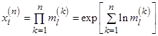follow a lognormal distribution, since follow Gaussian distribution for large n due to the central limit theorem. When can be either positive or negative, the distribution has lognormal tails. The most common case in computer simulations is r = 2, and the relevant cascade is often called binomial.

In the simplest version of the binomial cascade multipliers are fixed, i.e. ml = a for any odd l and ml = b for any even l. Often in the literature, this implementation is referred as an ab-model. When a + b = 1, the binomial model is called the canonical binomial cascade [Mandelbrot, 2001]. This variant of the model is fully deterministic, and thus the final realization xi can be described exactly for any given i and iteration number n. The deterministic structure of this model results in some artificial properties of the final data series. For example, when a > b, the first value in the final data series will always be the global maximum, and thus for large a values the record is showing a trend, in contrast to our expectations from real world complex systems.

The simplest way of introducing a random component into the ab-model is to choose randomly at each step, either odd or even multiplier will be a, then the remaining one will be b. Since for the canonical model b = 1 – a, the integral of the data series is preserved. For an example of the ab-model with randomly chosen multipliers, see Fig.1a.

a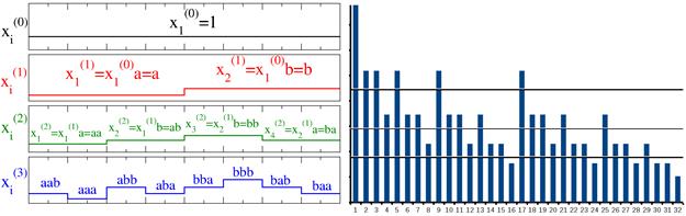 b

Fig. 1. Random ab-model synthesis algorithm (a); deterministic model realization for n = 5 (b)

Results.

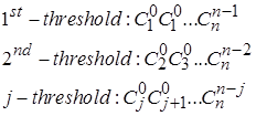
Next, the statistics of return intervals between events that exceed various thresholds Q have been analyzed, see Fig. 1b. An important indicator is the distribution of the return intervals for various thresholds. For the deterministic variant of the ab-model, only n–2 nontrivial thresholds are available.

Figure 2 shows that the histogram of the return intervals for the deterministic ab-model is given by the diagonals of the Pascal's triangle. To obtain the relevant histogram values, one has to remove the last element in each row of Pascal's triangle, i.e., at the right edge of the triangle a full line (containing of ones) should be eliminated. The original Pascal's triangle is shown in Fig. 2a, the modified triangle is shown in Fig. 2b. Line numbers in Fig. 2 refer to the number of iterations n in the binomial cascade model.

Let us assume n = 10. For the first nontrivial threshold (j = 1) the histogram values are: 1, 2, 3, 4, 5, 6, 7, 8, 9, 10, for the third threshold (j = 3) they are: 1, 4, 10, 20, 35, 56, 84, 120 (underlined on Fig. 2b).

a 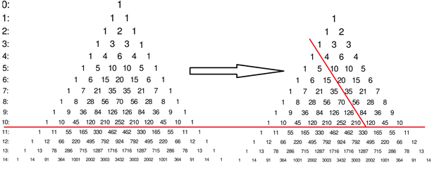b

Fig. 2. Pascal triangle

Each element of the triangle is a binomial coefficient. Thus histogram values for any given threshold can be described as:

The probability density function of return intervals PQ(τ) can be easily obtained as a normalized histogram and can be expressed as function of the threshold for τ > 1 as shown in Fig. 3. In Fig. 3 τ is return interval between peaks reduced by 1, TQ is the average interval τ for a certain threshold. The solid lines show the analytical solution according to Fig. 2, and the dotted line – the result of a numerical experiment for one realization obtained with n = 15. Good agreement of the simulation results with the proposed analytical solution indicate that it can be extrapolated to the randomized cascade model.

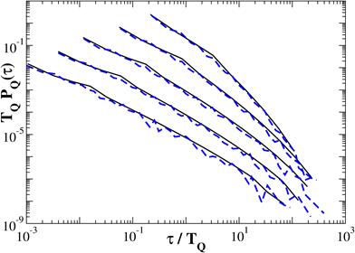
Fig. 3. Probability density function for analytical solution (black) and for numerical experiment (blue)

Conclusions.

It is known that the return interval statistics for randomized model are in good agreement with the data obtained in the biological structures and physiological processes analysis. Therefore using the proposed approach by varying the parameters n and j one can easily reproduce the relevant statistics for arbitrary n values ??without performing any numerical simulation. Since the solution can be extrapolated to whatever large n values, it can be used to avoid finite size effects. On the other hand when dealing with various numerical estimates by choosing relevant n values one can reproduce typical finite size effects for given data lengths. By comparing numerical and analytical results and running appropriate statistical tests, one can also estimate the probabilities that a deviation from cascade-like return interval distribution is due to finite size effects or is a result of the internal randomness in the studied dynamical system, that may be superimposed to the long-range dependent character of the data.

Acknowledgment.

This work have been supported by the Ministry of Education and Science of the Russian Federation (project 10.97.2011).

References.

Bogachev M.I., Kireenkov I.S., Nifontov E.M., Bunde A. Statistics of return intervals between large heartbeat intervals and their usability for prediction of disorders. // New Journal of Physics. 2009. Vol. 11. P. 063036 (1-18).

Huikuri H.V., Mäkikallio T.H., Perkiömäki J. Measurement of heart rate variability by methods based on nonlinear dynamics // J. Electrocardiol. 2003. Vol. 36. P. 95–99.

Ivanov P. Ch., Rosenblum M.G., Peng C.-K. et al. Scaling behaviour of heartbeat intervals obtained by wavelet-based time-series analysis // Nature (London). 1996. Vol. 383. P. 323-327.

Ivanov P. Ch. , Amaral L.A.N., Goldberger A.L. et al. Multifractality in human heartbeat dynamics // Nature (London). 1999. Vol. 399. P. 461 – 465.

Mandelbrot B.B. Gaussian Self-Affinity and Fractals. New York: Springer, 2001.

Peng C.-K., Buldyrev S. V. , Havlin S. et al. Mosaic organization of DNA nucleotides // Phys. Rev. E. 1994. Vol. 49. P. 1685–1689.

Sokolova A., Bogachev M.I., Bunde A. Clustering of ventricular arrhythmic complexes in heart rhythm // Phys. Rev. E. Vol. 83. 2011. P. 021918(1-7).

Yu Z.-G., Ahn V., Lau K.-S. Multifractal and correlation analyses of protein sequences from complete genomes. // Phys. Rev. E. 2003. Vol. 68. P. 021913 (1–10).